SAEs on AIDO.Cell: biological footprint

Published

April 21, 2026

First question: once you train an SAE on an scFM, do the features actually mean something biological? Or are they just compressed basis vectors with no preferred interpretation?

Setup

Model: AIDO.Cell-100M, layer 12 residual stream.
SAE: Top-k with k=32, 5120 features (8× overcomplete), trained on PBMC3K.
Feature → gene matrix \(\mathbf{F}\): mean activation of each feature across cells, pooled per gene. A feature’s “top genes” are the genes it activates most strongly.

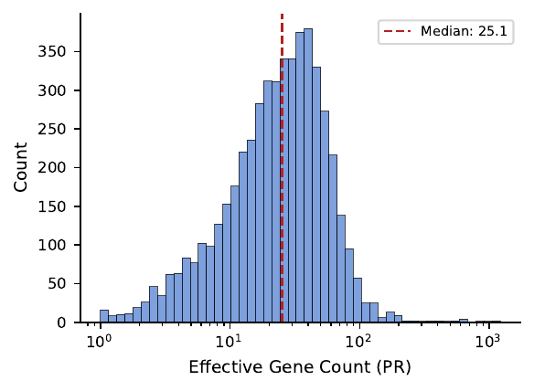
For each feature we ran GO enrichment on its top genes. Rather than picking an arbitrary top-N cutoff, we use the Participation Ratio (PR) as a feature-specific gene count:

\[ \mathrm{PR}_i = \frac{\left(\sum_j \mathbf{F}_{ij}^2\right)^2}{\sum_j \mathbf{F}_{ij}^4}. \]

PR is an effective count: ~1 if the feature is dominated by one gene, ~thousands if it spreads activation uniformly. Sharp features get narrow gene sets for enrichment; broad features get larger ones.

Distribution of PR across 5120 features. Median ≈ 25 genes; the long tail goes from single-gene features up to thousands.

Result 1 — Most features are biologically annotated

64% of SAE features get statistically significant GO enrichment at q < 0.05, vs ~34% for the raw AIDO.Cell neurons at the same layer. The SAE roughly doubles the fraction of axes that map to known biology.

Result 2 — SAE features are more specific

Annotation rate is a coarse metric — a feature could get significantly enriched for a generic term like “cellular process” and count as annotated. To measure specificity we used the maximum Information Content (IC) of each feature’s enriched GO terms (IC rewards terms that are informative in the GO DAG — rare leaves score high, broad roots score low).

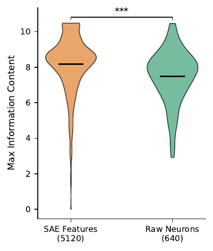
Max IC per feature, SAE vs raw layer-12 neurons. SAE features concentrate on more specific terms.

SAE features are shifted toward higher max IC (Mann-Whitney p < 0.001). They tend to be enriched for more specific biological concepts, not just broad ones.

Caveat — baseline choice matters. We also ran Independent Component Analysis (ICA) on the raw layer-12 activations as a linear-decomposition baseline. ICA gave nearly identical max-IC distributions to the SAE. So the specificity win is clearly over raw activations, not over all unsupervised decompositions. The SAE’s distinguishing advantage shows up elsewhere — in sparsity, feature compositionality, and (as the next posts show) in giving us manipulable axes.

Result 3 — features are mostly orthogonal, but cluster coherently

Pairwise gene-set overlap between features is tiny: 93% of feature pairs share zero top-activating genes. The dictionary covers distinct concepts.

The interesting structure is in the sparse tail. If we build a feature graph with edges where overlap > 0.2, the resulting connected components are biologically coherent: within-CC mean GO overlap is 0.247, vs 0.018 for all pairs — more than 10× enriched. Components correspond to broad programs (a Viral Defence cluster, a B-cell Signalling cluster, …) made of several features encoding sub-aspects of the same biology.

Example features

A few hits, to make this concrete:

F2685 — Aerobic respiration (broad cellular state).
F1480 — Cell cycle regulation (broad state).
F4590 — Germinal center formation (cell-type-specific, B-cell).
F3181 — Type I interferon signalling (cell-type-adjacent, antiviral program).
F4367 — Viral defence (used in the steering experiments).
F3170 — B-cell identity (used in the steering experiments).

Takeaway

The SAE basis is doing real work: it turns a polysemantic latent space into a dictionary where most axes correspond to specific biological programs. This is the prerequisite for everything that follows — without interpretable features, “steering a feature” would be meaningless.